Mechanics: 1-Dimensional Kinematics
1-D Kinematics: Problem Set Overview
There are 23 ready-to-use problem sets on the topic of 1-Dimensional Kinematics. The problems target your ability to use the average velocity and average acceleration equations, to interpret position-time and velocity-time graphs, and to use the kinematic equations to determine the answer to problems, including those which involve a free fall acceleration. Problems range in difficulty from the very easy and straight-forward to the very difficult and complex.
Average Speed, Average Velocity, and Average Acceleration Equations
The equations for average velocity (vave) and average acceleration (aave) are stated below.

The ∆time is the change in time over which the position change or velocity change is measured. When using a stopwatch to measure this time, the ∆time is simply the time reading on the stopwatch. We refer to this as t in the equations.
An inspection of these equations shows that there are clear mathematical relationships between the following sets of quantities:
From the top equation:
average velocity (vave), initial velocity (vi), final velocity (vf), displacement and time
From the bottom equation:
average acceleration (aave), initial velocity (vi), final velocity (vf) and time
Position-Time Graphs
Position-time graphs represent variations in an object's position over the course of time. Thus, an inspection of the values being plotted along the vertical axis allows one to determine position values and changes in position values. These axis values are related to the distance and displacement for an object's motion. The displacement of an object is simply the overall change in position; it considers only the initial and the final positions and ignores all in-between positions. Being a vector quantity, it includes a direction that is often expressed as a positive or a negative sign (e.g., + for rightward and - for leftward). The distance traveled by an object is the accumulation of all the ground covered. In effect, it is the sum of all the changes in position for each leg of a trip; such sums must ignore the + and - signs since distance is a scalar quantity. Being a scalar quantity, it is ignorant of direction and does not distinguish between a change in position to the left or to the right. If a person walks 2 meters, left and then 6 meters right, then the displacement is 4 meters to the right and the distance is 8 meters.
Slopes of such position-time graphs yield a ratio of the position change to time change for any specified interval of time. As such, the slopes are equivalent to the velocity of an object. Velocity (slope in this case) is a vector quantity that has a direction associated with it. Mathematically, the velocity direction is often represented by a positive or a negative value. Upward-sloping lines are associated with positive velocities and downward-sloping lines are associated with negative velocities. For a complex motion with multiple slopes, the average velocity can be determined by connecting the initial and final position and calculating the slope of the connecting line. Alternatively, the average velocity could be determined by reading the overall position change (displacement) off the axis and dividing by the change in time.
The average speed for any motion is simply the distance to time ratio. For a simple motion involving a constant velocity, the average speed is the absolute value of the slope. For a complex motion with several slopes, the average speed is the overall distance traveled divided by the time of travel. As mentioned above, the overall distance traveled can be determined by summing the absolute value of the individual position changes for each leg of the motion.
Velocity-Time Graphs
Velocity-time plots represent variations in an object's velocity over the course of time. As such, the slope of such graphs provides a velocity change to time change ratio; this ratio represents the acceleration of the object. Some of the questions in these problem sets will test your ability to use the coordinates for two points on a line to determine the slope. The slope is simply the change in the y coordinates divided by the change in the x-coordinate. You can use our video to learn more about the process.
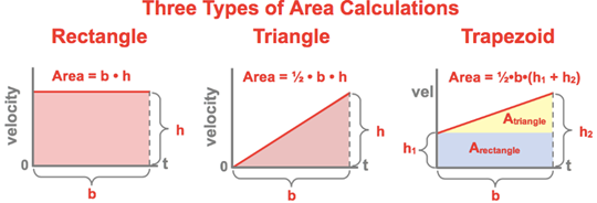
Velocity-time plots can also be used to determine the distance traveled by an object and the displacement of an object. The area between a plotted line and the time axis (which could be a positive or a negative value) represents the displacement of the object. The area spoken of here is formed by the plotted line, the time axis and two imaginary vertical lines drawn at two specified points in time. The resulting area could be represented by either a rectangle, a triangle, a trapezoid or a collection of such shapes. The graphic below depicts a variety of resulting shapes and the appropriate formulas for calculating areas from each of them.
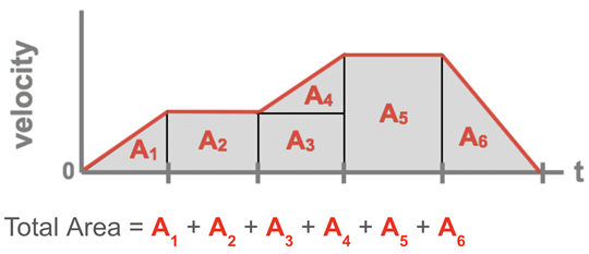
For a complex motion like that represented below, the total area can be broken into a collection of smaller shapes. The area of the individual sections can then be added together to determine the total area.
The Big Four - Kinematic Equations
Kinematics (the topic of the current unit) is the science of describing the motion of objects. An object's motion can be described using words, diagrams, numbers, graphs and equations. The most commonly used of all equations are the four kinematic equations - affectionately known as the big four. These four equations allow a student to make a prediction of how fast (velocity and speed), how far (displacement and distance), or how much time is required of an object during a motion. The four equations are listed below.
- d = vo • t + 0.5 • a • t2
 vf = vo + a • t
- vf2 = vo 2 + 2 • a • d
- d = (vo + vf)/ 2 • t
where
- d = displacement
- t = time
- a = acceleration
- vo = original or initial velocity
- vf = final velocity
Each of the above kinematic equations have four variables. The usefulness of the equations is that they allow a person to make a prediction about the value of one of the variables if given the value of three other variables. By knowing three, one can calculate a fourth. The problem-solving strategy used in this collection of problems will center around this idea. Each problem consists of a word-story problem in which information about an object's motion is given. The goal is to carefully read through each story problem to identify at least three pieces of known information in order to calculate a fourth requested piece of information. Often the known information is explicitly stated - "A car moving with an initial velocity of 23.4 m/s...". At other times there are statements included within the word problem such as "Starting from rest, ...? or "...comes to a stop." Such statements imply that the initial velocity is 0 m/s and the final velocity is 0 m/s (respectively).
While the equations are extremely useful, there is one condition which must be met in order for the equations to be used. The object under study must have a constant and uniform acceleration. If an object changes its acceleration at a given point during the motion such that it accelerates at one rate and then later accelerates at a second rate, then the motion must be divided into two phases and each phase must be analyzed separately.
Free Fall and Acceleration Caused by Gravity
Some of the problems in these problem sets involve free fall type motion. Free fall is a type of motion in which the only force acting upon the moving object is the force of gravity. When an object is in free fall, its motion is influenced solely by the force of gravity and the object accelerates at 9.8 m/s/s. The 9.8 m/s/s value is the acceleration of any free falling object irregardless of the characteristics of the object. Such an acceleration is dependent solely upon the gravitational characteristics of the planet and is thus called the acceleration of gravity or acceleration caused by gravity and represented by the variable g. While the value of g is 9.8 m/s/s on Earth, it is a different value on other planets where the gravitational characteristics are different. NOTE: Some classes use a rounded value of 10 m/s/s to simplify calculations.)
There are some unique aspects about the trajectory of a free falling object which are worth noting and serve very useful in one's approach to solving problems. Any object that is originally projected vertically upward and under the sole influenc of gravity will eventually reach a peak height before turning around and falling back downward. At the peak of the trajectory, the velocity of the object is momentarily 0 m/s. The time required to reach the peak is equal to the time required to fall from the peak back to its original position. The total time of flight is thus twice the time required to reach the peak. The velocity of the object one second prior to the peak is of the same magnitude as the velocity of the object one second after reaching the peak. And similarly, the velocity of the object two seconds prior to the peak is of the same magnitude as the velocity of the object two seconds after reaching the peak. You may find our video on Solving Free Fall Problems to be useful.
Habits of an Effective Problem-Solver
An effective problem solver by habit approaches a physics problem in a manner that reflects a collection of disciplined habits. While not every effective problem solver employs the same approach, they all have habits which they share in common. These habits are described briefly here. An effective problem-solver...
- ...reads the problem carefully and develops a mental picture of the physical situation. If needed, they sketch a simple diagram of the physical situation to help visualize it.
- ...identifies the known and unknown quantities in an organized manner, often times recording them on the diagram itself. They equate given values to the symbols used to represent the corresponding quantity (e.g., vo = 0 m/s, a = 2.67 m/s/s, vf = ???).
- ...plots a strategy for solving for the unknown quantity; the strategy will typically centers around the use of physics equations is heavily dependent upon an understanding of physics principles.
- ...identifies the appropriate formula(s) to use, often times writing them down. Where needed, they perform the needed conversion of quantities into the proper unit.
- ...performs substitutions and algebraic manipulations in order to solve for the unknown quantity.
Read more...
Additional Readings/Study Aids:
The following pages from The Physics Classroom tutorial may serve to be useful in assisting you in the understanding of the concepts and mathematics associated with these problems.
Watch a Video
We have developed and continue to develop Video Tutorials on introductory physics topics. You can find these videos on our YouTube channel. We have an entire Playlist on the topic of Kinematics.