Velocity-Time Graphs - Complete Toolkit
Objectives
-
To relate the shape (horizontal line, diagonal line, downward-sloping line, etc.) of a velocity-time graph to the motion of an object.
-
To relate the slope value of the line on a velocity-time graph at a given time or during a given period of time to the instantaneous or the average velocity of an object and to determine such velocity values using a slope calculation.
-
To relate the area between the line and the time-axis of a velocity-time graph to the displacement of the object and to determine such displacement values using an area calculation.
-
To relate the motion of an object as described by a velocity-time graph to other representations of an object's motion - dot diagrams, motion diagrams, tabular data, etc.
-
To analyze position-time graphs and transpose them into the corresponding velocity-time graphs (and vice versa).
Readings from The Physics Classroom Tutorial
-
The Physics Classroom Tutorial, 1D-Kinematics Chapter, Lesson 4
Interactive Simulations
-
Graph That Motion TPC's Shockwave Physics Studios
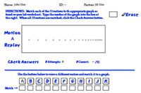 This activity challenges students to view 11 different animations and make an effort to match the animation to the appropriate position-time or velocity-time graph. Once 11 matches have been made, students can check their answers, receive feedback, and make adjustments. The activity is accompanied by a Directions page.
-
Two Stage Rocket TPC's Shockwave Physics Studios
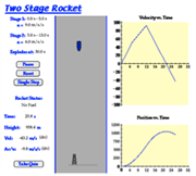 Students analyze the motion of a two-stage rocket, relating the slope and area calculations to the altitude and acceleration of the rocket. This simulation is accompanied by an activity sheet that guides students through the process:
-
Graph Matching Motion Model Simulation/computer Model
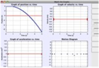 Powerful way to investigate the meaning of shape and slope for 3 types of motion graphs. To set it up correctly requires the student to analyze and interpret computer-generated motion of a blue object moving either with constant velocity or constant acceleration. Next, match the motion by using sliders to set initial position, velocity, and acceleration of an adjacent red object. Last, use sliders to predict the shape of the related velocity and acceleration graphs to give correct straight-line slopes.
-
PhET Teacher Contributions: Velocity vs. Time Graphs
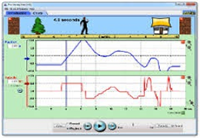 This ready-to-use lesson plan was developed specifically for use with the PhET simulation "The Moving Man". It’s designed to help beginning students differentiate velocity vs. time graphs from position vs. time graphs, and also to promote understanding of multiple frames of reference in analyzing an object's motion. Only basic graphing skills are required of the student. It was created by a high school teacher under the sponsorship of the PhET project. (NOTE: The simulation “The Moving Man” must be open and running in order to complete the lesson.)
Link to the companion simulation: http://phet.colorado.edu/en/simulation/moving-man
-
Car Race Model
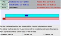 This customizable EJS model (Easy Java Simulation) is designed to help learners visualize the difference between constant velocity and constant acceleration. It features the classic physics scenario in kinematics: a lead car travels at constant velocity on a straight track while a second car moves from rest with constant acceleration in the same direction. Each time the game is reset, the position & velocity of each car change. Which car will win?
Video and Animations
-
Physlet Physics: Compare Position vs. Time and Velocity vs. Time Graphs
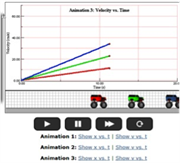 Three animations depict both P/T and V/T graphs for 3 Monster Trucks. By analyzing the animations, students reason about how initial position and the speed affects the shape of the graph. A printable worksheet accompanies the resource with conceptual questions and data tables for students to complete.
-
Physlet Physics: Average and Instantaneous Velocity
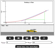 A follow-up to the “Average Velocity” Physlet, this exercise lets students set initial and final times to view rise, run, and slope. All values are automatically generated by the animation. The point of the exercise is to show graphically that, as the time interval gets smaller and smaller, the average velocity approaches the instantaneous velocity.
-
Physlet Physics: Determine the Correct Graph
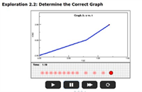 Given a dot diagram of a moving ball, students must identify the correct graph that matches up to the motion of the ball. First, they will choose the correct Position vs. Time graph, then the correct Velocity vs. Time graph. We like this resource because it prompts deeper reasoning about the shape of motion graphs and it uses multiple representations to gauge student understanding. It also includes a pdf worksheet that engages students in analyzing mistakes. Link to the worksheet:
-
Physlet Physics: Curtain Blocks Your View of the Golf Ball
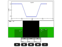 This animation shows a putted golf ball rolling along a green, but a black curtain blocks your view of the motion during mid-roll. A Velocity vs. Time graph is simultaneously displayed. Students will analyze the V/T graph to figure out the terrain of the green behind the curtain. First, they provide a written description of the motion, then click to view the animation without the curtain.
-
Physlet Physics: Set the x(t) of a Monster Truck
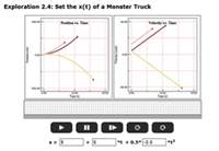 This short exercise packs lots of punch, as it lets students explore all 3 terms in the equation x = xo + vo•t + 1/2•a•t2. Set the initial conditions, then watch as both a P/T and V/T graph are generated. Change one of the variables, then see how the graph changes by clicking the box for “Multiple Graphs Superimposed”. The resource comes with a printable worksheet as well.
Labs and Investigations
-
The Physics Classroom, The Laboratory, Velocity-Time Graphs Lab
Using a motion detector, students explore the shapes of velocity-time graphs for various types of motion.
-
The Physics Classroom, The Laboratory, Match That Graph Lab
Students walk in front of a computer-interfaced motion detector in an effort to match a provided graph.
Minds On Physics Internet Modules:
The Minds On Physics Internet Modules are a collection of interactive questioning modules that target a student’s conceptual understanding. Each question is accompanied by detailed help that addresses the various components of the question.
-
Kinematic Graphing, Ass’t KG5 - Basics of v-t Graphs
-
Kinematic Graphing, Ass’t KG6 - Interpreting v-t Graphs (I)
-
Kinematic Graphing, Ass’t KG7 - Interpreting v-t Graphs (II)
-
Kinematic Graphing, Ass’t KG8 - Slope and Area of v-t Graphs
-
Kinematic Graphing, Ass’t KG9 - Graphs and Oil Drops DIagrams
-
Kinematic Graphing, Ass’t KG10 - Common Misconceptions
-
Kinematic Graphing, Ass’t KG11 - Matching p-t and v-t Graphs
Concept Building Exercises:
-
The Curriculum Corner, 1D Kinematics, Describing Motion with Velocity-Time Graphs
-
The Curriculum Corner, 1D Kinematics, Describing Motion Graphically
-
The Curriculum Corner, 1D Kinematics, Interpreting Velocity-Time Graphs
-
The Curriculum Corner, 1D Kinematics, Graphing Summary
Problem-Solving Exercises:
-
The Calculator Pad, 1-Dimensional Kinematics, Problems #13 - #17
Science Reasoning Activities:
-
The Physics Classroom: Science Reasoning Center, Kinematics
-
The Physics Classroom: Science Reasoning Center, Velocity-Time Graphs
Common Misconceptions and Difficulties:
-
Speeding Up and Slowing Down
A common misconception is to attribute speeding up to an upward-sloping line and slowing down to a downward-sloping line. This connection between slope and changes in speed only works for objects that have a positive velocity. If the line is located below the time axis, then a speeding up motion is a downward-sloping line and a slowing down motion is an upward-sloping line. It is useful to train students to associate speeding up with a line that gets further from the time axis and to associate slowing down with a line gets closer to the time axis.
-
Changing Directions
A common misconception that must be confronted pertains to the changing of direction of an object as represented on a velocity-time graph. Students often confuse the changing of direction of the line on the graph with a change in direction of the object. The direction an object is moving impacts whether the velocity value is positive or negative. This in turn affects the location of the line on the graph – above or below the time axis. An object that changes direction is thus represented by a line that passes across the time axis from above to below (or vice versa).
Related PER (Physics Education Research)
-
Kinematics Graph Interpretation Project
Recent work has uncovered a consistent set of student difficulties with graphs of position, velocity, and acceleration vs. time. For the busy teacher, this synopsis will be a quick read but worth every minute. It organizes the findings of several years of the Kinematics Graph Interpretation Project on one page.
-
Searching for Evidence of Student Understanding, T. Bartiromo, presented at the Physics Education Research Conference 2010, Portland, Oregon
This research examined whether high school students can translate between representations (an ability often considered to be an “expert trait” in solving physics problems). It also gauged whether requiring multiple representations for a single problem helped instructors better assess student understanding. It’s a short read (3.5 pages), and has interesting implications: “We can argue that by assessing students with multiple choice questions or by requiring only one representation, one might get a false sense of students’ mastery…..Therefore, assessments need to include problems in which students respond with more than one representation.”
Interactive Digital Homework Problem:
-
 Illinois PER Interactive Examples: v vs. t
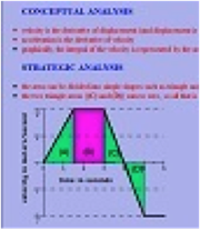
If you haven’t seen physicist Gary Gladding’s research-based homework problems, you’re in for a great surprise! This in-depth digital problem shows a V/T graph for a moving object and asks the student to find the final position. An explicit help sequence is provided for each step: 1) conceptual analysis, 2) recognize and choose appropriate strategies for problem-solving, and 3) do the math. Immediate feedback is received for both correct and incorrect responses (meaning kids can continue progressing with the problem solving even if they make a mistake along the way.)
Elsewhere on the Web:
-
Graph Sketching and Recognition
This page features 37 practice problems from The Physics Classroom pertains to both position-time and velocity-time graphs. Each problem is accompanied by an answer and a thorough explanation.
Standards:
A. Next Generation Science Standards (NGSS)
Note: The topic of kinematics is not directly covered in the NGSS.
B. Common Core Standards for Mathematics – Grades 9-12
Standards for Mathematical Practice
-
MP.2 Reason abstractly and quantitatively
-
MP.6 Attend to precision
-
MP.8 Look for and express regularity in repeated reasoning
Quantities: Reason Quantitatively and Use Units to Solve Problems
-
N-Q.1 Use units as a way to understand problems and to guide the solution of multi-step problems; choose and interpret units consistently in formulas; choose and interpret the scale and the origin in graphs and data displays.
-
N-Q.3 Choose a level of accuracy appropriate to limitations on measurement when reporting quantities.
Algebra: Seeing Structure in Expressions – Interpret the Structure of Expressions
-
A-SSE.1.a Interpret parts of an expression, such as terms, factors, and coefficients
-
A-SSE.2 Use the structure of an expression to identify ways to rewrite it.
Algebra: Creating Equations
-
A-CED.2 Create equations in two or more variables to represent relationships between quantities; graph equations on coordinate axes with labels and scales.
-
A-CED.4 Rearrange formulas to highlight a quantity of interest, using the same reasoning as in solving equations.
Functions: Interpret Functions that Arise in Terms of a Context
-
F-IF.4 For a function that models a relationship between two quantities, interpret key features of graphs and tables in terms of the quantities, and sketch graphs showing key features given a verbal description of the relationship.
-
F-IF.6 Calculate and interpret the average rate of change of a function (presented symbolically or as a table) over a specified interval. Estimate the rate of change from a graph.
Building Functions: Linear, Quadratic, and Exponential Models
-
F-LE.1.b Recognize situations in which one quantity changes at a constant rate per unit interval relative to another.
-
F-LE.1.c Recognize situations in which a quantity grows or decays by a constant percent rate per unit interval relative to another.
Functions: Interpret Expressions for Functions in Terms of the Situation They Model
-
F-LE.5 Interpret the parameters in a linear or exponential function in terms of a context.
Reading Level
This set of tutorials scored 57.47 on the Flesch-Kincaid Readability Index, corresponding with Grade 9. It scored 12.18 on the Gunning-Fog Index, which indicates the number of years of formal education a person requires in order to easily understand the text on the first reading (corresponding to Grade 12).
C. Common Core Standards for English/Language Arts (ELA) – Grades 9-12
Craft and Structure
-
RST.11-12.4 Determine the meaning of symbols, key terms, and other domain-specific words and phrases as they are used in a specific scientific or technical context relevant to grades 11-12 texts and topics.
Integration of Knowledge and Ideas
-
RST.11-12.9 Synthesize information from a range of sources (e.g., texts, experiments, simulations) into a coherent understanding of a process, phenomenon, or concept, resolving conflicting information when possible.
Range of Reading and Level of Text Complexity
-
RST.11.12.10 By the end of grade 12, read and comprehend science/technical texts in the grades 11-CCR text complexity band independently and proficiently.
D. College Ready Physics Standards (Heller and Stewart)
Essential Knowledge-Middle School
Constant and Changing Linear Motion
-
M.3.1.3 When the distance an object travels increases with each successive unit of time, it is speeding up; when the distance an object travels decreases with each successive unit of time, it is slowing down.
-
M.3.1.4 The relationship between distance and time is nonlinear when an object’s speed is changing and when it is moving in a series with different constant speeds.
-
The constant speed an object would travel to move the same distance in the same total time interval is the average speed.
-
Average speed can be represented and calculated from the mathematical representation (average speed – total distance traveled/total time interval), data tables, and the nonlinear Distance vs. Time graph.
-
For objects traveling to a final destination in a series of different constant speeds, the average speed is not the same as the average of the constant speeds.
Essential Knowledge: High School
Constant and Changing Linear Motion
-
H.3.1.1 The displacement, or change in position, of an object is a vector quantity that can be calculated by subtracting the initial position from the final position, where initial and final positions can have positive and negative values . Displacement is not always equal to the distance traveled.
-
H.3.1.2 An object that travels the same displacement in each successive unit time interval has constant velocity. Constant velocity is a vector quantity and can be represented by and calculated from a position versus time graph, a motion diagram or the mathematical representation for average velocity. The sign (+ or -) of the constant velocity indicates the direction of the velocity vector, which is the direction of motion.
-
H.3.1.3 The constant velocity an object would travel to achieve the same change in position in the same time interval, even when the object’s velocity is changing, is the average velocity for the time interval. Average velocity can be mathematically represented by vave = (xf - xi)/(tf - ti). For straight-line motion, average velocity can be represented by and calculated from the mathematical representation, a curved position versus time graph and a motion diagram.
-
H.3.1.4 The velocity of an object in straight-line motion changes continuously, from instant to instant while it is speeding up or slowing down and/or changing direction. The velocity of an object at any instant (clock reading) is called its instantaneous velocity. The object does not have this velocity over any time interval or travel any distance with this velocity. Instead, the instantaneous velocity is the constant velocity at which an object would continue to move if its motion stopped changing at that instant. An object with zero instantaneous velocity can be accelerating (e.g., motion up a ramp then back down the ramp).
-
H.3.1.5 When the change in an object’s instantaneous velocity is the same in each successive unit time interval, the object has constant acceleration. For straight-line motion, constant acceleration can be represented by and calculated from a linear instantaneous velocity versus time graph, a motion diagram and the mathematical representation [a = (vf - vi)/(tf - ti)]. The sign (+ or -) of the constant acceleration indicates the direction of the change-of-velocity vector. A negative sign does not necessarily mean that the object is traveling in the negative direction or that it is slowing down. [BOUNDARY: The term “deceleration” should be avoided because students tend to associate a negative sign of acceleration only with slowing down.]
Learning Outcomes
-
Represent and calculate the distance traveled by an object, as well as the displacement, the speed and the velocity of an object for different problems. Representations include data tables, distance versus time graphs, position versus time graphs, motion diagrams and their mathematical representations. Interpret the meaning of the sign (+ or -) of the displacement and velocity.
-
Investigate, and make a claim about the straight-line motion of an object in different laboratory situations. Representations include data tables, position versus time graphs, instantaneous velocity versus time graphs, motion diagrams, and their mathematical representations. When appropriate, calculate the constant velocity, average velocity or constant acceleration of the object. Interpret the meaning of the sign of the constant velocity, average velocity or constant acceleration. Interpret the meaning of the average velocity.
-
Explain what is “constant” when an object is moving with a constant velocity and how an object with a negative constant velocity is moving. Justify the explanation by constructing sketches of motion diagrams and using the shape of position and instantaneous velocity versus time graphs.
-
Explain what is “constant” when an object is moving with a constant acceleration, and explain the two ways in which an object that has a positive constant acceleration and a negative constant acceleration. Justify the explanations by constructing sketches of motion diagrams and using the shape of instantaneous velocity versus time graphs.
-
Compare and contrast the following: distance traveled and displacement; speed and velocity; constant velocity and instantaneous velocity; constant velocity and average velocity; and velocity and acceleration.
-
Translate between different representations of the motion of objects: verbal and/or written descriptions, motion diagrams, data tables, graphical representations (position versus time graphs and instantaneous velocity versus time graphs) and mathematical representations.